3.1. Introduction

This is a paper presenting noise in sounds, understood as random variations in time, and not (hopefully) unpleasant sounds. Nor is noise understood here as loud sounds, but instead as unvoiced sounds, i.e. sounds without a tonal quality.

Noise is inherent in all musical sounds, including the human voice. Without noise and random fluctuations, most sounds are dull, lifeless, and synthetic, and noise can indeed add a wide variety of tone qualities to a harmonic sound. The work presented here is undertaken as a first step in the investigation of the importance of noise in the perception of the timbre of musical sounds. Demonstrations (Audiostrations) show the importance of noise in many situations, and a 3D model of the noise space renders a large palette of sound categories.

Noise is an important part of much twentieth-century music, including the musique concrète of Schaeffer, the stochastic (random) processes of Xenakis, and the random selection of grains in granular synthesis. A selection of perception issues regarding noise is reviewed, including the perception of random pulses, the perception of pitch in noise and the sensation of pleasantness in tonal and non-tonal components.

Three types of noises and irregularities are identified: random events, unvoiced sounds, and harmonic sounds with amplitude and frequency irregularities. Random events are not investigated further in this work. Noise is seen, in a first step, as uncorrelated samples in time (throwing dice is an example of this), and therefore characterized only by its distribution, i.e. the probability that a certain sample value occurs. If the current sample of the noise is dependent on previous samples, it has a non-uniform spectral envelope (colored noise). This is the case for some percussive instruments, as well as whispering and unvoiced consonants, which are modeled well by filtered white noise. The second part of this work deals with sinusoids modulated with band-limited noise - either amplitude modulated (shimmer), or frequency modulated (jitter). If enough harmonics are summed together, this can model almost all voiced sounds, including string and wind instruments and the human voice. The noise parameters are visualized in two 3D manipulation interfaces, consisting of bandwidth, strength and correlation for the jitter and shimmer, respectively. The bandwidth is a measure of how fast the noise is changing, and the correlation is a measure of how much alike the noise is to the noise of another overtone. There is a dramatic difference in the timbre of the resulting sound in the different positions of this space; the shimmer is rumbling, windy, crackling, the jitter is rough, weird, walking. Audiostrations of the noise space are given to present the different categories, and finally, a 3D manipulation interface is presented.

3.2. Noise and Random Fluctuations

The distinction between noise and tone has been clear for a long time. Helmholtz (1954) provides the following definition: The sensation of a musical tone is due to a rapid periodic motion of the sonorous body; the sensation of noise to non-periodic motions. He then proceeds to study the former in his On the Sensation of Tone. Schaeffer (1966) did not consider the temporal form different for noise or voiced sounds. These forms were used indifferently for harmonic sounds and filtered white noises, although, white noise is the exact opposition of the harmonic sound, since it occupies the entire spectrum. In between harmonic sounds and white noise, Schaeffer placed the cymbal, group of cymbals, group of gongs, bells, etc, and chords.

The futurists proposed, without success it seems (Chadabe, 1997), a series of instruments, the intonarumori, that produced rumbles, whispers, creaks, and other noises. Schaeffer went on to collaborate with Pierre Henry on musique concrete, in which recorded sounds, many of them unvoiced, were used in the compositions. Stockhausen and others used electronic generators, sinusoids and white noise in their early works. Another composer, Xenakis, used stochastic processes not only in compositions, but also in the creation of new sounds. The distinction between composition and sound events have been blurred in granular synthesis (Truax, 1994) - a method in which long music pieces can be obtained by random summation of time or frequency shifted short (10-50 ms) grains, often extracted from a short sampled waveform using a random selection process.

For the purpose of this paper, three types of noise and random irregularities have been found, random pulses, unvoiced sounds, and voiced sounds with random irregularities added to the amplitudes and frequencies. Pierce (2001) differentiates slow random pulses, which are heard as separate pulses, from pulses occurring at the rate of a few hundred pulses per second, where not all pulses are detected individually. Above this, a smooth noise is heard, with no individual pulses perceivable. No further analysis of the random pulses will be made in this paper.

Dannenbring and Bregman (1990) showed that bandpass-filtered noises produced stream segregation (two alternating sounds heard as two separate streams). Warren (1999) used repeated static Gaussian noises (frozen noise) to show the perception of infrapitch (very low frequency pitch). His conclusions (on the accompanying Audio CD) are that repetition of frozen noise segments renders a whooshing, motorboating, and noisy pitch, dependent on the repetition rate. For the low infrapitch (2 Hz), a collection of rattles, clangs and other metallic types of sounds may also be perceived, in addition to the whooshing sound.

Audiostration 1 [] Frozen Noise Repetitions. In this sound, the infrapitch sound is slowly transformed from whooshing to motorboat to noisy pitch.

Other methods for obtaining a pitch sensation from noise, as stated in (Roads, 1996), include amplitude modulating, or delaying and adding the noise (comb filter noise).

Zwicker (1999) tested tonality (a feature distinguishing noise and tone quality of sounds) versus sensory pleasantness (a complex sensation that is influenced by elementary auditory sensations such as roughness, sharpness, tonality and loudness) and found a strong dependency, indicating that band-pass filtered noise with large bandwidth have low relative pleasantness, as compared to sinusoids and band-pass filtered noise with low bandwidth.

3.3. Noise in Musical Sounds

Noise and irregularities are common in many musical instruments. Indeed, without some irregularity, the sound produced by most musical instruments would become synthetic, lacking the life that is necessary to produce an enjoyable sound. Noise is found in its purest form in some percussive instruments, and in particular in the unvoiced consonants of the human voice. In addition, blowing instruments, such as the flute, have an additive noise component. Struck and plucked string instruments, such as the piano and the guitar often have unvoiced plucking and striking noises, whereas the bowed instruments have aperiodicities that add to the quality of the instruments.

A short survey of some of the noise sources in musical instruments is given here. Recall that noise is understood as unvoiced sounds without a clear tonal quality, or as random variations on the overtones amplitudes and frequencies. Often, of course, the noise and the voiced components exist together, such as in the voiced consonants.

For more information about the mechanical and physical properties of musical instruments, see for instance (Rossing et al., 2001). More information about the signal processing methods used in the analysis/synthesis part can be found in (Roads, 1996).

Whereas most musical instruments do have a noise component, either continuous or transient-like, that is caused by the physical behavior of the instrument, the effect of playing on continuous-control instruments (Jensen, 2002a) is dominant concerning the random fluctuations of the sound. This is of much importance in the perception of sounds, and it is an important part of most played musical sounds (Jensen, 1999). The examples of instruments given below are mainly found in classical Western music. Most types are also found in other cultures, and the statements given here generally also apply to these instruments.

Analysis/Synthesis

For the case of unvoiced sounds, the sounds can be modeled as white noise, filtered by a filter that restitutes the temporal and tone quality of the sound. In order to test this hypothesis, a simple experiment has been designed. In the analysis/synthesis experiment, the original sound is split into short segments (23 ms, with 12 ms overlap) and the filter coefficients are estimated from all segments. The structure of the experiment is shown in Figure 1.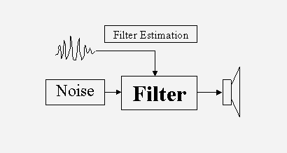

Different filter estimation methods have been tested; but the linear predictive coding (Proakis & Manolakis, 1996) was found to perform best. In this method, the filter shape is adjusted so the excitation noise is having as uniform a spectrum as possible. Therefore the noise input to the filter is white noise (i.e. having the same energy for all frequency bands).

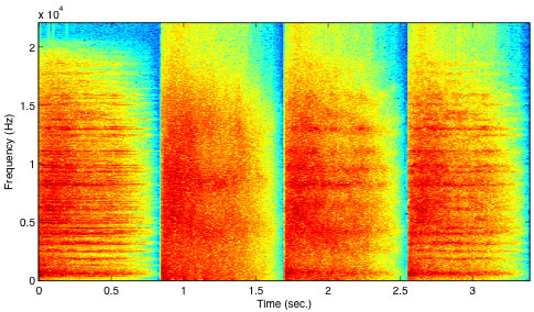
3.3.2. Consonants and Whispering

The human voice is an extraordinary instrument that can combine voiced sounds or constriction noise from open vocal cords (whispering) with different tongue and teeth constriction noises (consonants). The consonants are defined by their articulatory features - place (position of the constriction) and manner (stops or fricatives). Whispers must -understandably, since most spoken information is retained in a whisper - be modeled through a time-varying filter-bank, which restitutes most of the shape of the spectral envelope (which defines the tone of the sound at a given instance). The consonants are modeled by a simpler spectral envelope than the whisper, since it has not been filtered by the vocal tract. Since the human voice is one of the most expressive instruments, a few experiments have been performed to see what filter shape is necessary to faithfully reproduce the unvoiced sound. A short segment consisting of whispering and consonants was recorded and modeled as white noise filtered with a 10, 30 and 100 filter coefficient filter. 100 filter coefficients were found necessary to restitute the full quality of the sound. This is illustrated in Figure 3, in which the formants visible in the original sound (between 0-2 seconds) only become visible when 100 filter coefficients are used (between 6-8 seconds).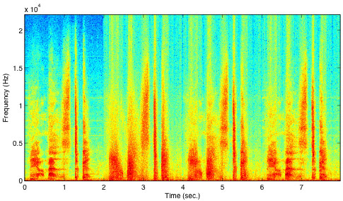

Figure 3 Spectrum of whisper and consonants, after analysis/synthesis. Original, 10, 30 and 100 filter coefficients.

Audiostration 3 [] Whisper and consonants.

3.3.3. Flute and Bowed Instruments

Flute
Many wind instruments have a noise component originating from the wind turbulences that occur while blowing. This is particularly true for the flute, where the noise component sometimes seems to be as strong as the voiced component. Other wind instruments with prominent blowing noise include the saxophone, if played soft. Since the flute sound always consists of the noise and the tone combined, the analysis/synthesis method of figure 1 does not work. Instead, the flute sound can be restituted with the harmonic noise model below, as shown in (Jensen, 1999). Ystad and Voinier (2001) modeled the flute by inserting noise into a waveguide model. The waveguide models the wave propagation in strings and tubes through delays and reflection filters. This is also known as the Karplus-Strong model (Roads, 1996).

Bowed Instruments
The bowed instruments all have a noise quality to the produced sounds. A stick and slip process governs the string when the bow is moving. The string stick to the bow until the tensions force that pulls the string back to the normal position exceeds the friction force between the bow and the string. This occurs after the waves introduced to the string have traveled one round trip (Rossing et al, 2001). This produces, in theory, a perfectly harmonic sound. There are, however, aperiodicities in the waveform of the bowed instruments (McIntyre et al. 1981), mainly originating from differences in the exact time when the slipping occurs. These aperiodicities render a sometimes rough, sometimes rich, and sometimes noisy sound, which are important qualities in the bowed musical instrument sounds.

3.4. Parameters of Noise

Noise is random samples in time. The values of these samples are dependent on the model of the noise, and the parameters of the model. The model is generally chosen to be uniform or Gaussian, which affects the likelihood that different values occur. Uniform corresponds to a normal dice, while Gaussian corresponds to a dice where 3 and 4 are more likely to occur than 1, 2, 5 and 6. The amplitude scaling and shifting are then the only parameters in white noise. If the samples are allowed to be dependent, i.e. that one random sample is determined, not only from a new random value, but also from a linear sum of previous or future samples, it has a non-uniform spectral envelope, and the noise is colored. If the spectral envelope is band-limited, then the noise can also be frequency shifted with a perceptual effect.

Distribution

The distribution affects how likely a value is. Common distributions are the uniform distribution, in which are values are equally likely, and the Gaussian distribution, in which the probability function is bell-shaped. In this work, a Gaussian model is assumed. This signifies that the values are normal-distributed, that is, that it is more likely to have a value around the mean than a different value. The Gaussian distributed noise is defined by its mean value and its standard deviation (corresponding to the level). These values are called the first and second moment, where the third moment is called skewness, and the fourth moment is called kurtosis. An illustration of the four moments of the Gaussian distribution is given in Figure 4.

The distribution is not believed to have a large influence on the sound. Although the difference between a uniform and a Gaussian distribution is audible, it is somehow difficult to make controlled experiments, because of the subtlety of the difference. The skewness and kurtosis are not believed to have a large perceptual effect either. In addition, in an analysis/synthesis situation, where the noise is to be recreated from a given sound, the higher order moments are more subject to estimation errors. The white noise used in the following is therefore Gaussian-distributed, with zero skewness and kurtosis.

Amplitude Scaling and Shifting

The amplitude scaling affects the loudness of the noise, whereas the shifting does not have a perceptual effect, except a potential click in the beginning and the end. Scaling the amplitude is the same as changing the standard deviation, and shifting is the same as changing the mean value.

Spectral Envelope

The spectral envelope, i.e. the tone of the noise, is an important attribute, as it can, for instance, change white noise into a whisper. In this work, a simple model for the spectral envelope is needed; therefore each sample value is set to be the weighted sum of a new random value and the previous sample:

(1)

where s(t) is the current sample, s(t-1) the previous sample, fc the filter coefficient, and rnd a new random value. The resulting filter shape is low-pass, which signifies that the high frequencies, the treble, is removed, and the low frequencies, the bass, is retained. In practice, the resulting noise samples needs to be normalized in amplitude. The filter coefficient fc can be found from the 3dB bandwidth value BW through the following formula

(2)

where sr is the sample rate. The constants are a function of the (arbitrary) –3dB cut-off frequency choice. The bandwidth is a more intuitive parameter than the filter coefficient, which doesn’t have a physical or perceptual signification.

Frequency Shifting

The frequency shifting is here performed by adding the filtered noise to the parameters of a sinusoidal. The noise can be added to the amplitude, in which case it is called shimmer, or to the frequency, in which case it is called jitter, or both

(3)

where σs and σj are the shimmer and jitter standard deviation, respectively, and ss and sj are the Gaussian low-pass filtered random samples. The amplitude a affects the loudness of the sinusoid. The amplitude modulation (shimmer) creates two sidebands of noise on each side of the center frequency f, and the frequency modulation (jitter) creates an infinity of sidebands, whose amplitude values are determined by a Bessel function. In practice, the infinity number of sidebands is giving a different tone to the jitter than the shimmer. The jitter is rendering low-frequency random pitch variations, when the bandwidth is low, and adding a rough quality to the sinusoidal, when the bandwidth is high. In contrast, the shimmer renders a rumbling quality to the sound for low bandwidths, and adds an additive noise, when the bandwidth is high.

3.5. Harmonic Shimmer and Jitter

If more sinusoids with harmonic frequencies

(4)

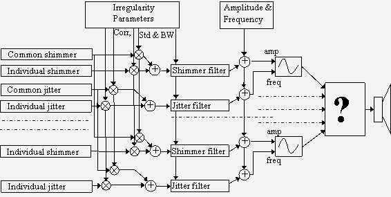
are added, a harmonic sound is obtained. Depending on the relative amplitude, the sound is more or less bright. Dependent on the attack and decay rise and fall time the sound will get more or less hard and percussive. This is not the issue here, however. Instead, the shimmer and jitter are added to all the sinusoids, with individual or common shimmer and jitter parameters for each partial (fundamental or overtone). The parameters are the same as in equation 3, except that there is a new parameter corresponding to the correlation of the noise between the overtones and the fundamental

(5)

where c is the correlation, s0 is the fundamental filtered noise, and sk is the filtered noise for the current overtone k. The x denotes shimmer or jitter. This model has previously been shown to model many musical instruments faithfully (Jensen, 1999), with individual noise parameter values for each overtone. In this work, however, the noise parameters are common to all overtones. This simplifies the visualization and manipulation of the model parameters, while at the same time still permitting a large variety of sound categories. The harmonic noise model is shown in Figure 5.

Figure 5 Structure of harmonic noise model.

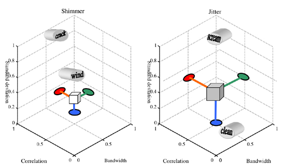
Standard Deviation

The standard deviation (std) affects the amount of noise, or irregularities on the overtones. If both the shimmer and jitter standard deviation values are zero, then the resulting sound is clean or calm, whereas, when the shimmer standard deviation is increased, the sound becomes agitated, and when the jitter standard deviation is increased, the sound becomes dirty. The jitter std values are generally found between 0.001-0.1 in common musical sounds. The shimmer std values are about ten times larger. These values are dependent on the overtone index and fundamental frequency, as well as on the musical instrument.

Bandwidth

The bandwidth of the shimmer and jitter noises for harmonic sounds gives approximately the same effect as with a single sinusoid. The effect of more overtones changes the relative effect, however. The jitter effect seems to get stronger with more overtones, whereas the shimmer effect seems to get weaker. The low bandwidth jitter sounds have random pitch, and are schizophrenic. The low shimmer bandwidth sounds are windy, or have random fluctuations. High bandwidth shimmer gives a dark additive noise, or an almost splashing quality, whereas the jitter becomes rough, almost screaming.

Correlation

The correlation is a rather interesting parameter in the harmonic model, as it renders a large variety of different tones, together with the bandwidth and standard deviation. Setting the correlation coefficient c low and the bandwidth high renders a rather dark additive noise quality to the shimmer, whereas the jitter renders a more nasal quality. As the correlation is increased, still with high bandwidth, the shimmer gets a different tone, almost splashing, whereas the jitter becomes somehow more insisting, almost screaming. As the bandwidth is decreased, still with high correlation, the shimmer goes towards a crackling quality, ending in a peaceful random fluctuation. The jitter goes through several categories of rough, full qualities, ending in random pitch. Finally, as the correlation is now decreased, the shimmer goes from the fluctuating sound to a beautiful windy quality, and the jitter gives a more schizophrenic sound. The correlation values in musical sounds are generally found between 0.25 and 0.75.

Discussion

The distinctions between the different noise parameter values never mask the underlying harmonic sound (unless the standard deviation is put that high), which has tone, hardness, percussiveness and other timbre attributes (Jensen, 2002b), independent of the shimmer and jitter, but the differences between the noise categories nevertheless seems clear in all cases. These subjective qualities may be individual, or at least subject to some variations between listeners, although it is believed that the perception of these sounds is common to most listeners. The verbal attributes used here is an attempt to communicate the perceptual meaning of the different parameter changes. It seems clear that there exist categories in the noise space, but no certainty exists as to the commonality of these categories.

3.6. Noise Model Manipulation

This section presents a graphical interface for the control of the parameters of the noise model. It has been found that three dimensions is the maximum controllable in one interface. Therefore the interface comprises two 3D plots, one for the shimmer, and one for the jitter. Each interface controls the standard deviation, bandwidth and correlation.

Interface Design

The model has been found through experimentation and research in the literature on interface design. Ware (2000) states, Object displays will be most effective when the components of the objects have a natural or metaphorical relationship to the data being represented. This includes, in particular, using depth cues, such as perspective cues (size), occlusion, depth of focus and shadows. Proximity luminance covariance is another cue, in which distant objects fade to the background color. Artificial spatial cues, such as dropped lines on ground planes are also effective in increasing the perception of position. Fitts’ law, which states that the selection time is proportional to the ratio of the distance to the size, can also be helpful in designing interfaces, as can the power law of practice (time of nth trial is proportional to the time of first trial minus the trial number times the steepness of the learning curve). To encourage skill learning, the interface should provide stimulus-response compatibility, i.e. have rapid and clear feedback.

Some of the spatial navigation metaphors are given in (Ware, 2000) to be world in hand (objective interface), eyeball in hand (subjective interface), walking and flying. The navigation in space is facilitated by the inclusion of landmarks, districts and paths, and overview maps, with user location and direction. Spatial distortion, such as intelligent zoom, in which areas in focus are expanded, can also be helpful.

Tufte (2001) investigates issues of graphical excellence, i.e. how well the data is shown, how much space it takes, how well the data is revealed in different levels of details, and how it encourages the eye to compare different sets of data. This is done through examples and analysis of distortion (lie factor), the data-ink ratio (no redundant information in the graphs), the use of a grid, data density and issues of aesthetics in data displays.

Some of these results are used in the following to make a useful interface for the manipulation of the noise parameters.

Parameters

The parameters of the noise model are, as depicted in figure 5, the standard deviation, bandwidth and correlation of the shimmer and jitter, respectively, where the standard deviation changes the sounds from a clean to an agitated (shimmer) or dirty (jitter) sound. Bandwidth affects the roughness, random pitch fluctuations, the windy quality and the dark noise quality. Correlation affects the crackling, or windy quality, or the additive quality of the noise (shimmer) and the screaming, or schizophrenic quality of the sound (jitter). Other verbal attributes of the sounds obtained include weird, rumbling, walking. In order to facilitate the visualization and manipulation task, all three parameters have been normalized between zero and one. The correlation was already defined to have this range, and the bandwidth is divided by the maximum bandwidth, the Nyquist frequency (sample rate divided by two), and the standard deviations are divided by the maximum allowed value.

Visualization and Manipulation

The visualization is done through two graphs, one corresponding to the shimmer, and one to the jitter. This is illustrated in Figure 6.

Figure 6 Prototype of the noise manipulation space. All three parameters have been normalized.

The noise parameters, represented by the square noise anchor, are modified by grabbing the dropped line anchors at the ground planes. A point to be noted about the interface is that the size and color intensity is a function of the distance of the object, which is helpful when trying to assert the position of the noise anchor. The landmarks in the interface (clean, wind, etc) are helpful when navigating through the space, both in understanding the effects of going in these directions, but also for rapid navigation, since pressing on a landmark will change the noise parameters to these values. The interface is shown here in the world in hand metaphor model. More navigation possibilities is believed to exist in the eye in hand metaphor model, but no experiments have been performed to assert this.

Audiostration 4 [] Serial harmonic noise. In these sounds, different parameters of the noise model are varied randomly. The parameters that are modified are the standard deviation (STD), bandwidth (BW) and correlation (CO) of the shimmer and jitter. In addition, each sound has a random length, between 1/4 and 2 seconds. Two separate streams of approximately one minute and a half have been produced, to produce a stereo file. The fundamental frequency (440 Hz), attack and decay, and brightness are not varied in the sounds.

3.7. Conclusions

This work has presented issues regarding noise, irregularities and random fluctuations in sounds. Based on an analysis of common random processes in musical sounds, two different noise types have been investigated: on the one hand the unvoiced sounds of certain percussive instruments and the whispering and consonants of the human voice, and on the other hand the deviations from the clean harmonic sound caused by random variations in the amplitude and frequencies of the overtones. The first noise is adequately modeled by a filtered white noise, the filter coefficients of which can be found through standard methods. The second type of noise is modeled by a harmonic noise model, in which the individual overtone frequencies and amplitudes are modulated by a random noise component. There are three parameters for the random amplitude (shimmer) and frequency (jitter) modulation respectively, standard deviation (strength), bandwidth (how fast the noise values change) and correlations (how alike the noise of an overtone is to the noise of the fundamental). The effect of the different parameters is noticeable - although it generally does not alter the basic perception (brightness, hardness, percussiveness), it brings splashing, windy, screaming, crackling, and all sorts of categories to the sound. Based on an analysis of interface design a manipulation and visualization interface is presented, in which ground-plane anchors are used to navigate with the help of perspective cues and landmarks. This is an introductory work whose long-term aim is to identify the categories of noise, so that these sounds can be used more easily in musical context.